An introduction to Reproducing Kernel Hilbert Spaces

A very common task in machine learning involves comparing complicated objects or distributions. These comparisons take many forms:

• Are datasets $P$ and $Q$ drawn from the same underlying distribution?
• Training generative models: where $\mathcal{X}$ is a set of samples from $P$, we might want to generate samples $Q$ that look like $P$.
• Does the model fit the observed data (goodness of fit)?
• Independence: given samples from the joint distribution $P_{XY}$, are X and Y independent?

A kernel encodes a comparison $k(x,y)$ between inputs. This choice defines a space of functions, which can then be used to answer some of the preceding questions. Moreover, not everything (cats, dogs) are vector like objects. A feature map that encodes the properties of these objects can then be acted on by kernels.

Define a feature map $\phi$, which maps inputs $X$ to a Hilbert space (a normed inner product space containing Cauchy sequence limits) $\mathcal{H}$.

The kernel is the inner product between the outputs of two vectors produced by the feature map: $$k(x,y)=\langle\phi(x),\phi(y)\rangle_{\mathcal{H}}$$

From this view, a kernel is a measure of similarity. It does not correspond to a distance or probability measure, but represents similar geometries in the space mapped out by the feature map.

A single kernel can have multiple feature maps, e.g. for $\phi_1(x)=x$ and $\phi_2(x)=\left(\frac{x}{\sqrt{2}},\frac{x}{\sqrt{2}}\right)$. Essentially, the representation does not need to be unique, whereas the kernel's design specifies the inner product of the Hilbert space.

It's easy to build new kernels from old ones: non-negative multiples or sums are kernels. Applying a mapping between spaces, then using a kernel gives you a kernel on the original inputs. These rules can be applied to give, say, polynomial kernels of the form $\left(\langle x, y\rangle)+c\right)^m$, which simply expands into a sum of products.

A reproducing kernel Hilbert space has elements $f:X\rightarrow\mathbb{R}$, which are functions. It has an additional property: evaluating $f(.)$ at any input must be bounded, to guarantee that the function cannot take arbitrarily large values at fixed points.

The kernel for an RKHS provides a function for each point: $k(\cdot,z)$. This gives the reproducing property: $$\langle f, k(\cdot,z)\rangle_{\mathcal{H}}=f(z)$$

In other words, the inner product of a function $f$ with the special kernel function centred at $z$ gives $f(z)$. In other words, the feature vector $\phi(z)$ can be taken to be the function $k(\cdot,z)$, which maps a new input $x$ to its similarity with $z$. Depending on current utility, you can treat the same object as a feature vector or a function. In the special case where $f=k(\cdot,x)$, $k(x,y)$ is then trivially the inner product between the two "similarity-to-this-point" functions. Imagine a Gaussian kernel, which has a bump centred at $x$ an $y$. Their RKHS product (and kernel value) is high if they are nearby, and lower if they are distant. This measure of similarity depends on the inner product of the RKHS, not just a simple convolution of the two bumps.

Consider the problem of XOR. You cannot draw a linear decision boundary in the input plane. The feature map $\phi(x)=(x_1,x_2,x_1x_2)$ lifts the input plane into a space where a plane separates the classes. For inputs encoded with $x_1,x_2\in\{-1,+1\}$, the weight vector $(0,0,1)$ gives $\langle(0,0,1),\phi(x)\rangle=x_1x_2$: XOR points have a negative score, and the decision boundary is the plane $z=0$ in feature space.

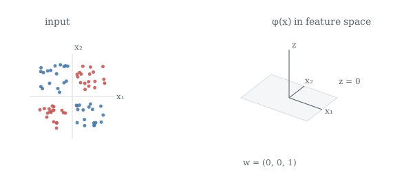
More generally, introduce a function $f(x)=\langle f,\phi(x)\rangle$. $f$ is an object, whereas $f(x)$ is the value taken at that point. The RKHS generalises this to a space, selecting an inner product so that $f(x)$ is computed as an inner product of $f$ with the feature representation of $x$. In a space with infinite dimensions, this allows us to work with kernel values rather than infinitely many feature coordinates.

Now, an infinite dimensional space implies an infinite feature dictionary. How do we select features then? We need rules for the combinations that are acceptable, e.g. a norm on functional space for convergence. And we want to penalise for less costly combinations of features. One desirable property is that the features should lie in $l_2$ space such that $\sum_{l=1}^{\infty}f_l^2<\infty$.

Consider a function composing features and feature maps $f(x)=\sum_{l=1}^{\infty}f_l\phi_l(x)$. And consider a finite combination of feature vectors at observed inputs, $f=\sum_{i=1}^m \alpha_i\phi(x_i)$. This has a coordinate in direction $l$, denoted $f_l=\sum_{i=1}^m \alpha_i\phi_l(x_i)$.

We can evaluate $f$ at $x$, giving us $$f(x)=\langle f,\phi(x)\rangle=\sum_{i=1}^m\alpha_i\langle\phi(x_i),\phi(x)\rangle=\sum_{i=1}^m\alpha_i k(x_i,x)$$

So each observed point contributes a kernel function $k(x_i,\cdot)$, weighted by $\alpha_i$. This hides the infinite feature coordinates inside each evaluation of the kernel. Note that not every function in the RKHS has to be a kernel section like $k(x_i,\cdot)$.

Smoothness and norms

The geometry of function space relates to practical fitting by providing a measure of cost. This is, in essence, regularisation: you want to fit the data whilst keeping a small RKHS norm.

In a set of infinite features, the later directions of the dictionary become rougher, and the kernel gives them smaller weights. A bounded RKHS norm thus requires the function's coefficients in those directions to be small - i.e. you can have rough elements, but it'll be expensive.

An example is the Fourier series $f(x)=\sum_{l=-\infty}^{\infty}\hat{f}_l \exp{(ilx)}$.

Consider the top-hat function. Its Fourier series builds a rectangular pulse from smooth waves:

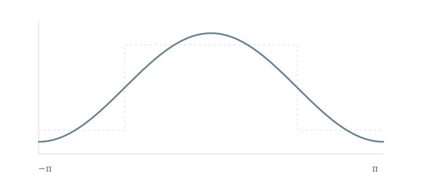
At the discontinuities, the Gibbs phenomenon leaves a small overshoot even as more frequencies are added. The coefficients also decay slower than those of a smoother function.

Consider a translation-invariant kernel, $k(x,y)=k(x-y)$. This kernel itself has a Fourier expansion, $k(x-y)=\sum_l \hat{k}_l\exp{(il(x-y))}$. For non-negative spectral weights $\hat{k}_l$, you can factor this into frequencies scaled by the weights' square-root. The usual $l_2$ inner product weights each Fourier component evenly. Instead, the RKHS inner product weights them according to the kernel $$\langle f,g\rangle$_{\mathcal{H}}=\sum_l\frac{\hat{f}_l\bar{\hat{g}_l}}{\hat{k}_l},\;||f||^2_{\mathcal{H}}=\sum_l\frac{|\hat{f}_l|^2}{\hat{k}_l}$$

If the kernel coefficients decay quickly at higher frequencies, then high frequency components are expensive. This is smoothness penalty in Fourier space. This is akin to a low pass filter. You can also have arbitrarily selective kernels, that remove high-frequency noise, e.g. 60Hz/50Hz line noise in EEGs. Moreover, by having an RKHS penalty in Fourier space (instead of a grid - which requires a kernel matrix), you can use the $\mathcal{O}(N\log N)$ Fast Fourier Transform to evaluate RKHS models on huge datasets. In the theoretical analysis of infinitely wide neural nets, during training they can be described as kernel machines governed by the neural tangent kernel. RKHS analysis in Fourier space found the spectral bias: neural nets learn the low-frequency smooth functions first, and this is explained by the Fourier penalty.